A DNN combines learned transformations; training adjusts parameters, and unseen examples establish whether it learned useful patterns.
If you give a computer thousands of labeled examples, how does it turn them into a useful prediction? The answer becomes much less mysterious when you follow one number through a neural network. Inputs are multiplied by weights, combined with biases, transformed, and passed onward. Training adjusts those weights and biases so the predictions better match the objective you supplied.
A deep neural network, or DNN, repeats these transformations through multiple learned layers. This article focuses on the foundation: what the layers do, how learning happens, and how to tell whether the result is useful. The diagrams and arithmetic are teaching examples, not reported experiments. You can open each picture at full size.
AI, machine learning, and deep learning
Artificial intelligence is a broad field. Some systems use explicit rules, search, or planning. Machine learning builds models whose behavior depends on patterns learned from data. Deep learning uses neural networks with multiple learned layers. A DNN is therefore one approach within AI; the terms do not all mean the same thing.
Think of sorting incoming support messages. A rule might flag every message containing a particular word. A learned classifier can use several signals together. The challenge is to learn patterns that remain useful when the wording changes. A sophisticated architecture will still struggle if the labels are inconsistent or the task is poorly defined.
For this guide, imagine predicting whether a message needs urgent handling. We will use simplified numerical features so you can see the calculations. A real system would require suitable examples, a clear urgency policy, and evaluation before use.
The picture: inputs, hidden layers, and output
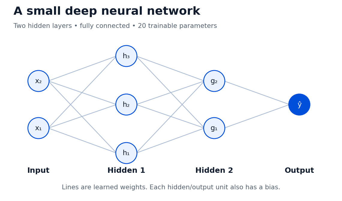
The input is a numerical representation of an example. The hidden layers produce intermediate representations. The output supplies the quantity needed by the task. In a dense layer, each output unit combines all the incoming features [1]. A hidden unit is a mathematical operation; the diagram does not claim it reproduces a biological neuron.
In this pictured network, two input values become three hidden activations, then two more, then one output. Each layer provides a new representation that the following layer can use. Depth refers to the sequence of learned transformations; width refers to the number of units in a layer.
There is no universally useful rule that more depth always wins. Ask whether extra capacity improves performance on examples the model did not learn from. A small model that generalizes can be more valuable than a large one that memorizes.
One neuron, calculated by hand
A dense unit computes a weighted sum, adds a bias, and applies an activation. Keras expresses the dense-layer operation as an activation applied to a dot product plus bias [1]. Here is an original numerical example:
x₁ = 2       w₁ = 0.5
x₂ = 1       w₂ = −1
b = 0.2

z = w₁x₁ + w₂x₂ + b
  = (0.5 × 2) + (−1 × 1) + 0.2
  = 0.2

a = ReLU(z) = max(0, 0.2) = 0.2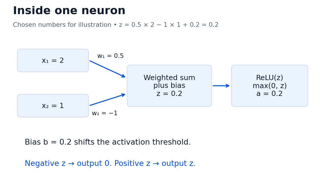
The weight tells you how a change in an incoming value affects this unit's sum, holding the other values fixed. A positive weight increases the sum when its input rises; a negative weight decreases it. Bias provides an offset, allowing the unit's activation threshold to move.
Do not interpret the negative weight here as a universal conclusion about an urgent message. These numbers were chosen to explain arithmetic. In a trained network, a weight's meaning depends on feature scaling, the other weights, and the rest of the computation. A single coefficient is rarely a complete explanation of a deep model.
Why activations matter
ReLU keeps positive values and replaces negative values with zero. Sigmoid maps values into the interval from zero to one. Softmax converts a vector of scores into nonnegative values summing to one. These functions serve different purposes [2].
The important idea is nonlinearity. Stacking affine transformations without nonlinear activations still produces one affine transformation. Activations let a network represent more complicated relationships: one feature may matter differently depending on another feature, and a decision boundary can bend.
For a binary classifier, one sigmoid output is a common design. For mutually exclusive classes, a vector of logits with a suitable softmax-based loss is common. For regression, an unconstrained numerical output may fit the task. Match the output and loss together; a probability-shaped number is not automatically a well-calibrated probability.
Parameters, activations, and hyperparameters
These three words are easy to mix up. Parameters are learned values such as weights and biases. Activations are intermediate values computed for a particular input. Hyperparameters are choices that shape training or architecture, such as layer width, batch size, or learning rate.
The small network in the first picture has 20 trainable parameters:
Swipe or scroll sideways to see every column.
| Layer | Weights | Biases | Total |
|---|---|---|---|
| Two inputs to three units | 2 × 3 = 6 | 3 | 9 |
| Three units to two units | 3 × 2 = 6 | 2 | 8 |
| Two units to one output | 2 × 1 = 2 | 1 | 3 |
| Entire pictured network | 14 | 6 | 20 |
The dense-layer counting rule is incoming features × outgoing units, plus one bias per outgoing unit when biases are enabled [1]. The input values themselves are not trainable parameters in this example.
A network can reuse the same parameters for many examples while producing different activations for each one. That distinction also explains why model weights and runtime memory are different quantities: processing inputs requires temporary working values in addition to stored parameters.
Forward propagation: making a prediction
The forward pass is the calculation from input toward output. Each layer receives the previous layer's activations and produces new ones. The final result might be a class score, several class scores, or a predicted measurement [3].
Suppose the urgent-message classifier produces 0.8. That number is useful only when you know its interpretation, the threshold used to take action, and the model's behavior on representative examples. A threshold of 0.5 is a choice, not a law of nature. Missing an urgent message and unnecessarily escalating an ordinary one may have different costs.
At this point the network has made a prediction. It has not necessarily learned anything from that prediction. Learning requires an objective and an update procedure.
Loss: telling the model what to improve
Loss is the numerical objective training tries to reduce. Mean squared error is common for numerical prediction; cross-entropy is common for classification [4]. The correct choice depends on the task and how the output is represented.
Here is a small regression example with deliberately chosen numbers:
Target y = 1
Prediction ŷ = 0.4
Squared error = (0.4 − 1)² = 0.36
An optimizer does not know that your real goal is “help the support team.” It follows the objective you defined. If your labels reward a shortcut, the network may learn the shortcut. If the training data rarely includes important exceptions, a low average loss may hide poor performance on those exceptions.
Metrics answer additional questions. Accuracy counts correct classifications under a decision rule. Precision describes how many positive predictions were right. Recall describes how many actual positive cases were found. Your loss, metrics, and acceptance standard should describe the same practical problem without being treated as interchangeable.
Backpropagation: finding the effect of each parameter
Backpropagation computes gradients: how the loss changes with respect to parameters. It applies the chain rule through the computational graph. TensorFlow's automatic differentiation tools record operations and calculate the corresponding derivatives [5]. The optimizer then uses gradients to update the parameters.
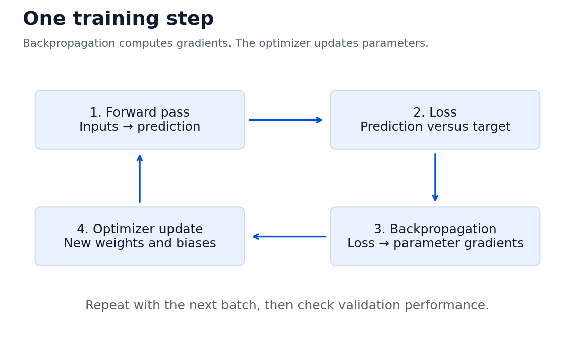
To see the direction of an update without a whole network, use one scalar weight:
Prediction: ŷ = w × x
Loss: L = ½(ŷ − y)²

x = 2, y = 1, w = 0.2
ŷ = 0.4
L = ½(0.4 − 1)² = 0.18

dL/dw = (wx − y) × x
      = (0.4 − 1) × 2 = −1.2

Learning rate η = 0.1
w_new = w − η(dL/dw)
      = 0.2 − 0.1(−1.2) = 0.32

New prediction = 0.32 × 2 = 0.64
New loss = ½(0.64 − 1)² = 0.0648
The loss decreases for this particular example and update. A negative gradient made gradient descent increase the weight. A positive gradient would make it decrease the weight. In a DNN, gradients also travel through the intervening layers and activations. The arithmetic becomes larger, but the local question remains: how does this parameter affect the loss?
This example does not prove that every training step decreases loss. Mini-batches, noisy data, curvature, and step size can all affect the result. Nor does a decrease on one training example establish better generalization.
Optimizers, learning rate, batches, and epochs
Gradient descent subtracts a learning-rate-scaled gradient. Optimizers such as SGD and Adam implement update strategies; Adam uses moving estimates of gradients and squared gradients [6]. Backpropagation computes the information used by the update, while the optimizer performs the update.
The learning rate controls step size. A very large step can overshoot; a very small step can make progress slow. Its usefulness depends on the optimizer and the rest of the training setup. There is no single best number for every network.
A batch is a group of examples processed for an update. An epoch is approximately one pass through the training dataset. If you have 1,000 examples and a batch size of 100, a straightforward setup makes 10 updates per epoch. Data sampling and incomplete final batches can change the details.
Record these choices so the result is interpretable. “Trained for 20 epochs” says much less without dataset size, batch size, optimizer, learning rate, and the checkpoint-selection rule.
Learning patterns without memorizing the answers
Training data is used to learn parameters. Validation data helps select models and settings. Test data is reserved for a final assessment. Fit preprocessing on training data, then apply the learned transformation to validation and test data; fitting it on all data can leak information [7].
Underfitting means the model has not captured useful structure well enough. Overfitting means training performance improves while performance on unseen examples fails to improve or worsens. TensorFlow's guide illustrates the tradeoff and methods such as regularization and dropout [8].
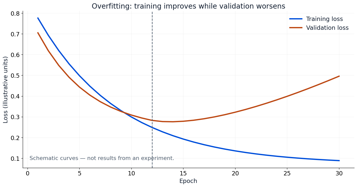
The practical question is what the validation examples represent. Randomly splitting near-duplicate messages may give an optimistic assessment. If deployment concerns later time periods, consider a time-based split. If several records belong to one person or organization, ensure your split matches whether new entities will appear at deployment.
Regularization can discourage excessively flexible fitting. Dropout changes the training computation by randomly dropping activations under its configured rules. Early stopping can select a checkpoint before validation performance deteriorates. None of these repairs incorrect labels or a test set that does not represent the intended use.
Data, scaling, and stable training
A numerical feature with a large range can dominate an unscaled input. Inspect units and distributions, and use preprocessing appropriate to the model and data. Save the fitted preprocessing alongside the network so inference uses the same transformation [7].
Check missing values and duplicate records before training. A model can exploit accidental clues, such as a label-related filename or a field created after the outcome. Such clues can disappear in real use. Better-looking metrics then describe an easier, unintended task.
Initialization also matters. Setting every unit in a layer to the same values can prevent units from learning distinct roles. Poor initialization and repeated transformations can contribute to gradients becoming too small or too large. Sensible initialization and training diagnostics help detect the problem [9].
A useful troubleshooting order is practical: inspect the data and objective, verify the input/output shapes, try to learn a tiny subset, check gradients and loss, then investigate architecture and optimization. Adding layers before understanding a broken pipeline usually makes diagnosis harder.
A small implementation to inspect
This Keras architecture matches the first diagram: two input features, hidden layers with three and two units, and one sigmoid output. It contains 20 parameters. The code defines the network; it does not report a trained result [10].
import keras
from keras import layers

model = keras.Sequential([
    keras.Input(shape=(2,)),
    layers.Dense(3, activation="relu"),
    layers.Dense(2, activation="relu"),
    layers.Dense(1, activation="sigmoid"),
])

model.compile(
    optimizer=keras.optimizers.Adam(learning_rate=0.001),
    loss="binary_crossentropy",
    metrics=["accuracy"],
)

model.summary()
# Training needs appropriately prepared features and labels.
# A larger real task may need a different architecture.
Read each line as a decision. The input has two features. ReLU introduces nonlinear transformations. The final sigmoid matches a binary probability-style output. Binary cross-entropy matches that output choice. Accuracy is one metric; it may be insufficient when classes are imbalanced or errors have unequal costs.
Before calling fit, establish your split and preprocessing. Before claiming success, evaluate against a baseline and inspect mistakes. The most valuable output of a beginner experiment is often a clear explanation of why it fails on certain examples.
The vocabulary to remember
Swipe or scroll sideways to see every column.
| Concept | Meaning in this guide |
|---|---|
| Feature | An input value representing part of an example. |
| Weight | A learned multiplier in the computation. |
| Bias | A learned offset. |
| Activation | A computed intermediate value, often after a nonlinear function. |
| Hidden layer | An intermediate learned transformation. |
| Logit | An output score before probability conversion. |
| Loss | The numerical training objective. |
| Gradient | A derivative describing sensitivity to a parameter. |
| Backpropagation | Calculating derivatives through the network. |
| Optimizer | Applying parameter updates using gradients. |
| Batch | Examples grouped for a training update. |
| Epoch | Approximately one pass through the training data. |
| Generalization | Useful performance on examples outside the training set. |
| Inference | Using a trained model to calculate outputs. |
How to continue learning
Start with the neuron calculation and parameter-count table. Then change one number and recompute the result. Next, follow the scalar gradient example until the sign of the update makes sense. Only then expand to a small training problem with a separate validation set.
The linked resources offer complementary routes: Keras documents operations and implementation; TensorFlow explains differentiation and generalization; Dive into Deep Learning develops the mathematics; scikit-learn explains evaluation pitfalls. Read the resource for the question you are trying to answer rather than opening every chapter at once.
My view for Saud Alotaibi’s Opinions is that the most useful understanding of a DNN connects three things: the calculation it performs, the objective that adjusts it, and the evidence that it works on new examples. Understanding one without the other two leaves a large part of the story missing.
Sources & further reading
- [1] Keras: Dense layer
- [2] Keras: activation functions
- [3] Dive into Deep Learning: multilayer perceptrons
- [4] Keras: loss functions
- [5] TensorFlow: gradients and automatic differentiation
- [6] Keras: optimizers
- [7] scikit-learn: common pitfalls and data leakage
- [8] TensorFlow: overfitting and underfitting
- [9] Dive into Deep Learning: numerical stability and initialization
- [10] Keras: the Sequential model